• Project Summary
• Problem Statement
• End User
• Data
• Methodology
  • Green Space Detection
  • Land Surface Temperature
  • Water Consumption
  • Seasonal Analysis
• Interface
• The Application
• How it Works
  • Data Preparation and Precomputation
  • Interactive Visualisation and Analysis
• Appendix
  • Causal Interpretation Warning
  • Data Limitations
  • SMA Model Coverage
• References

Project Summary

This project develops an interactive web application to assess green space loss and related environmental impacts in the Las Vegas Valley. In the context of recent tension around regional policy to remove “nonfunctional” turf, the application visualizes local changes in green space alongside shifts in land surface temperature and water consumption. A map-based dashboard enables tract-level exploration of spatial patterns and temporal change. By linking policy implementation to measurable landscape changes, the project directly supports more informed evaluation of its impact on water conservation and environmental conditions.

Problem Statement

The Colorado River Basin, a system providing water to millions across the southwestern US, is in crisis: runoff into the basin continues to decline while consumption levels remain constant. To reduce water consumption across the Las Vegas Valley, Assembly Bill 356 was passed in 2021, prohibiting the use of water from the basin to irrigate “nonfunctional” turf (green space with no clear purpose) by the start of 2027. In January 2026, a group of residents sued the Southern Nevada Water Authority (SNWA), claiming that the removal of these green spaces have led to negative downstream environmental effects. While existing tools offer residents and policymakers fragmented views of the related data, our application brings all of these variables together in one accessible interface, allowing users to connect policy implementation with measurable change at a hyper-local level.

End User

This dashboard is designed for Las Vegas Valley policymakers and residents, including those involved in ongoing litigation. Analysis has shown that turf irrigation in the region requires substantial amounts of water, especially when compared to more sustainable landscaping alternatives. But getting rid of the turf to reduce water consumption has considerable tradeoffs: academic research has demonstrated that removing nonfunctional turf leads to net local warming. Compiling turf loss with surface temperature and water consumption estimates allows residents and policymakers to view changes and patterns over time at a local level. The dashboard, thus, becomes a tool in which legal arguments can be grounded in measurable environmental evidence.

Data

Category	Dataset	Description	Source
GEE	Sentinel-2	Monthly median spectral band values from Copernicus Sentinel-2 MSI surface reflectance at 10m resolution, cloud-masked with gap-filling from prior months.	Link
	Land Surface Temperature	Monthly median land surface temperature from Landsat 8 thermal infrared (Band 10) at 30m resolution, cloud-masked and converted to Celsius with gap-filling from prior months.	Link
	Evapotranspiration	Monthly actual evapotranspiration at 30m resolution from OpenET, combining six satellite-based models (DisALEXI, eeMETRIC, geeSEBAL, PT-JPL, SIMS, SSEBop) into a single ensemble estimate.	Link
	Census Tract Boundaries	Census tract boundaries for tracts within the Las Vegas Valley.	Link
Other	Metro Area Boundary	Las Vegas Valley boundary compiled using Las Vegas - Henderson and Boulder City.	Link

Methodology

Green Space Detection

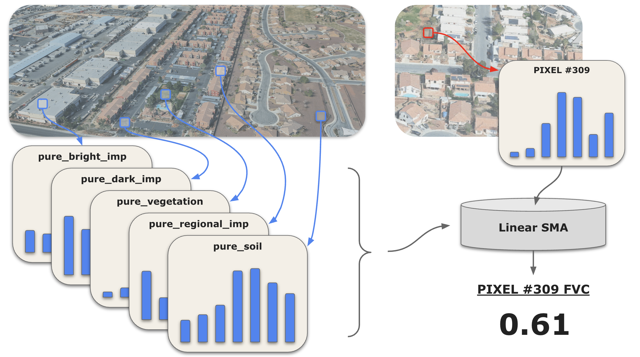
An office park may cover a cluster of several Sentinel-2 pixels, a median strip may run a narrow trail through a few pixels, and a roundabout may cover just a small fraction of one pixel. To identify changes to turf of varying sizes, we estimate fractional vegetation cover (FVC) using a 5-endmember linear spectral mixture analysis (SMA) model. This model approximates the fractional coverage of each endmember within a pixel, and we then isolate the calculated vegetation percentages to arrive at our pixel-level FVC estimates.

SMA model overview. The composition of any pixel (here, a random pixel #309) is estimated using 5 endmembers: 1) green vegetation, 2) soil 3) dark impervious materials (e.g. asphalt), 4) bright impervious materials (e.g. concrete), and 5) regional impervious materials (e.g. terra cotta roofing).

FVC Estimation Code

// =============================================================================
// CONFIGURATION
// =============================================================================
 
var startYear = 2019;
var startMonth = 1;
var endYear = 2025;
var endMonth = 12;
var baselineYear = 2019;
 
var bands = ['B2', 'B3', 'B4', 'B8', 'B8A', 'B11', 'B12'];
 
// Reference image date range (for endmember extraction)
var refStartDate = ee.Date.fromYMD(2022, 6, 1);
var refEndDate = ee.Date.fromYMD(2022, 7, 1);

// =============================================================================
// LOAD BOUNDARY
// =============================================================================
 
var lv_metro_boundary = ee.FeatureCollection('projects/lv-turf-removal/assets/lv_metro_boundary');

// =============================================================================
// HELPER FUNCTIONS
// =============================================================================
 
/**
 * Masks clouds, cirrus, and cloud shadows from Sentinel-2 imagery
 * Uses QA60 band for clouds/cirrus and SCL band for cloud shadows
 */
function maskS2clouds(image) {
  // QA60 band for clouds and cirrus
  var qa = image.select('QA60');
  var cloudBitMask = 1 << 10;
  var cirrusBitMask = 1 << 11;
 
  var qaMask = qa.bitwiseAnd(cloudBitMask).eq(0)
      .and(qa.bitwiseAnd(cirrusBitMask).eq(0));
  
  // SCL band for cloud shadows (and optionally other classes)
  // SCL values: 3 = cloud shadow, 8 = cloud medium prob, 9 = cloud high prob, 10 = cirrus
  var scl = image.select('SCL');
  var sclMask = scl.neq(3)   // cloud shadow
      .and(scl.neq(8))       // cloud medium probability
      .and(scl.neq(9))       // cloud high probability
      .and(scl.neq(10));     // cirrus
  
  // Combine both masks
  var combinedMask = qaMask.and(sclMask);
 
  return image.updateMask(combinedMask).divide(10000);
}
 
/**
 * Gets median spectral profile for a geometry from the reference image
 */
var getProfile = function(geometry, refImg) {
  var dict = refImg.reduceRegion({
    reducer: ee.Reducer.median(),
    geometry: geometry,
    scale: 10,
    maxPixels: 1e9
  });
  return bands.map(function(b) { return dict.get(b); });
};
 
/**
 * Performs spectral unmixing and calculates RMSE
 */
function unmixWithRMSE(img, endmembers) {
  var unmixed = img.unmix(endmembers, true, true)
    .rename(['veg', 'npv', 'bimp', 'dimp', 'tcr']);
    
  // RMSE calculation
  var fractionArray = unmixed.toArray().toArray(1);
  var endmemberArray = ee.Array(endmembers).transpose();
  
  var reconstructedArray = ee.Image(endmemberArray).matrixMultiply(fractionArray);
  var reconstructed = reconstructedArray
    .arrayProject([0])
    .arrayFlatten([bands]);
    
  var error = img.subtract(reconstructed).pow(2);
  var rmse = error.reduce(ee.Reducer.mean()).sqrt().rename('rmse');
  
  return unmixed.addBands(rmse);
}

// =============================================================================
// CREATE MONTHLY COMPOSITES
// =============================================================================
 
var startDate = ee.Date.fromYMD(startYear, startMonth, 1);
var endDate = ee.Date.fromYMD(endYear, endMonth, 1);
var nMonths = endDate.difference(startDate, 'month').round();
 
// Create a fully masked placeholder image with correct band structure
var maskedPlaceholder = ee.Image.constant(ee.List.repeat(0, bands.length))
  .rename(bands)
  .updateMask(0)
  .clip(lv_metro_boundary);
 
// Create raw monthly composites (may have gaps due to clouds)
var rawMonthlyComposites = ee.ImageCollection.fromImages(
  ee.List.sequence(0, nMonths).map(function(n) {
    var currentStart = startDate.advance(n, 'month');
    var currentEnd = currentStart.advance(1, 'month');
    
    var collection = ee.ImageCollection("COPERNICUS/S2_SR_HARMONIZED")
      .filterBounds(lv_metro_boundary)
      .filterDate(currentStart, currentEnd)
      .filter(ee.Filter.lt('CLOUDY_PIXEL_PERCENTAGE', 20))
      .map(maskS2clouds);
    
    // Check if collection has any images
    var hasImages = collection.size().gt(0);
    
    // Use median composite if images exist, otherwise use masked placeholder
    var composite = ee.Image(ee.Algorithms.If(
      hasImages,
      collection.median().select(bands).clip(lv_metro_boundary),
      maskedPlaceholder
    ));
      
    return composite.set({
      'month': currentStart.get('month'),
      'year': currentStart.get('year'),
      'system:time_start': currentStart.millis()
    });
  })
);

// =============================================================================
// GAP-FILL MISSING MONTHS (carry forward values from previous month)
// =============================================================================
 
var compositeList = rawMonthlyComposites.toList(rawMonthlyComposites.size());
 
var filledList = ee.List(
  ee.List.sequence(0, nMonths).iterate(function(n, acc) {
    n = ee.Number(n);
    acc = ee.List(acc);
 
    var current = ee.Image(compositeList.get(n));
    
    // Check if current image has ANY valid pixels
    var validPixelCount = current.select(0).reduceRegion({
      reducer: ee.Reducer.count(),
      geometry: lv_metro_boundary,
      scale: 1000,  // Coarse scale for efficiency
      maxPixels: 1e6
    }).get(bands[0]);
    
    var hasValidPixels = ee.Number(validPixelCount).gt(0);
 
    var filled = ee.Algorithms.If(
      n.gt(0),
      ee.Algorithms.If(
        hasValidPixels,
        // Current has some valid pixels: fill any remaining gaps with previous
        current.unmask(ee.Image(acc.get(n.subtract(1)))),
        // Current is entirely empty: use previous month entirely
        ee.Image(acc.get(n.subtract(1)))
      ),
      current
    );
 
    return acc.add(ee.Image(filled));
  }, ee.List([]))
);
 
// Reconstruct ImageCollection with preserved metadata
var monthlyComposites = ee.ImageCollection.fromImages(
  ee.List.sequence(0, nMonths).map(function(n) {
    var filledImg = ee.Image(filledList.get(n));
    var originalImg = ee.Image(compositeList.get(n));
    
    return filledImg.copyProperties(originalImg, ['month', 'year', 'system:time_start']);
  })
);

// =============================================================================
// CREATE REFERENCE IMAGE AND ENDMEMBERS
// =============================================================================
 
var referenceImg = ee.ImageCollection("COPERNICUS/S2_SR_HARMONIZED")
  .filterBounds(lv_metro_boundary)
  .filterDate(refStartDate, refEndDate)
  .filter(ee.Filter.lt('CLOUDY_PIXEL_PERCENTAGE', 20))
  .map(maskS2clouds)
  .median()
  .select(bands)
  .clip(lv_metro_boundary);
 
// em1_veg, em2_npv, etc.
var endmembers = [
  getProfile(em1_veg, referenceImg),
  getProfile(em2_npv, referenceImg),
  getProfile(em3_bimp, referenceImg),
  getProfile(em4_dimp, referenceImg),
  getProfile(em5_tcr, referenceImg)
];

// =============================================================================
// SPECTRAL UNMIXING WITH RMSE
// =============================================================================
 
var unmixedCollection = monthlyComposites.map(function(img) {
  return unmixWithRMSE(img, endmembers)
    .copyProperties(img, ['system:time_start', 'month', 'year']);
});

// =============================================================================
// CALCULATE VEGETATION DIFFERENCE FROM BASELINE
// =============================================================================
 
var baselineCollection = unmixedCollection.filter(ee.Filter.eq('year', baselineYear));
 
var monthJoin = ee.Join.saveFirst({ matchKey: 'baseline_img' });
var filterByMonth = ee.Filter.equals({ leftField: 'month', rightField: 'month' });
 
var joinedCollection = ee.ImageCollection(
  monthJoin.apply(unmixedCollection, baselineCollection, filterByMonth)
);
 
var diffCollection = joinedCollection.map(function(img) {
  var currentImg = ee.Image(img);
  var baselineImg = ee.Image(currentImg.get('baseline_img'));
  
  var currentVeg = currentImg.select('veg');
  var baselineVeg = baselineImg.select('veg');
  
  var diff = currentVeg.subtract(baselineVeg).rename('veg_diff');
  
  return currentImg.addBands(diff);
});

// =============================================================================
// COMPUTE RMSE
// =============================================================================
 
var monthNames = ['Jan', 'Feb', 'Mar', 'Apr', 'May', 'Jun', 'Jul', 'Aug', 'Sep', 'Oct', 'Nov', 'Dec'];
 
// Calculate mean RMSE for each calendar month across all years
var monthlyRMSEValues = ee.List.sequence(1, 12).map(function(month) {
  var monthImages = unmixedCollection.filter(ee.Filter.eq('month', month));
  var meanMSE = monthImages.select('rmse')
    .map(function(img) { return img.pow(2); })
    .mean();
  
  return ee.Number(meanMSE.reduceRegion({
    reducer: ee.Reducer.mean(),
    geometry: lv_metro_boundary,
    scale: 100,
    maxPixels: 1e9
  }).get('rmse')).sqrt();
});
 
// Create ordered dictionary (Jan -> Dec)
var monthlyRMSEDict = ee.Dictionary.fromLists(monthNames, monthlyRMSEValues);
print('Monthly RMSE:');
print(monthlyRMSEDict);
 
// Calculate total (overall) RMSE across all images
var totalRMSE = unmixedCollection.select('rmse')
  .map(function(img) { return img.pow(2); })
  .mean()
  .reduceRegion({
    reducer: ee.Reducer.mean(),
    geometry: lv_metro_boundary,
    scale: 100,
    maxPixels: 1e9
  });

var globalRMSE = ee.Number(totalRMSE.get('rmse')).sqrt();
print('Global RMSE:');
print(globalRMSE);

Land Surface Temperature

Land surface temperature (LST) is brought in using pre-computed estimates from Landsat 8 Collection 2 Level 2 dataset.

Water Consumption

In arid regions like Las Vegas, evapotranspiration (ET) serves as a strong proxy for water consumption: with minimal rainfall, almost all ET is the result of irrigation. ET is modeled by combining satellite-derived land surface temperature and vegetation indices with meteorological variables such as wind speed, humidity, and solar radiation. The resulting value measures the total flux of water from the land surface to the atmosphere through both soil evaporation and plant transpiration.

Water Consumption Estimation Code

// =================================================================
// 1. SETUP & CONFIGURATION
// =================================================================

var lasvegas_boundary = ee.FeatureCollection('projects/project-ba3da252-127d-4b0d-bf0/assets/lasvegas_boundary');
var roi = lasvegas_boundary.geometry();

var CONFIG = {
  runExport: true, 
  startYear: 2019,
  endYear: 2025,
  assetFolder: 'projects/yg-casa-project-11365/assets/water_monthly_collection/',
  scale: 30,
  ensembleId: "projects/openet/assets/ensemble/conus/gridmet/monthly/v2_1",
  ssebopId: "projects/openet/assets/ssebop/conus/gridmet/monthly/v2_1"
};

// =================================================================
// 2. PRE-CALCULATE 2019 BASELINE
// =================================================================

var ensembleCol = ee.ImageCollection(CONFIG.ensembleId);
var ssebopCol = ee.ImageCollection(CONFIG.ssebopId);
var months = ee.List.sequence(1, 12);

var baseline2019 = months.map(function(m) {
  var start = ee.Date.fromYMD(2019, m, 1);
  var end = start.advance(1, 'month');
  var img = ensembleCol.filterDate(start, end)
    .filterBounds(roi)
    .select('et_ensemble_mad')
    .mean()
    .clip(roi);
  return img.set('month', m);
});

var baseline2019Col = ee.ImageCollection.fromImages(baseline2019);

// =================================================================
// 3. GENERATE MULTI-BAND COLLECTION (2019-2025)
// =================================================================

var years = ee.List.sequence(CONFIG.startYear, CONFIG.endYear);

var etCollection = ee.ImageCollection.fromImages(years.map(function(y) {
  return months.map(function(m) {
    var startDate = ee.Date.fromYMD(y, m, 1);
    var endDate = startDate.advance(1, 'month');
    
    var isBefore2025 = ee.Number(y).lt(2025);
    var currentCollection = ee.ImageCollection(ee.Algorithms.If(isBefore2025, ensembleCol, ssebopCol));
    var bandToSelect = ee.Algorithms.If(isBefore2025, 'et_ensemble_mad', 'et');
    
    // 1. Get current month ET
    var img = currentCollection.filterDate(startDate, endDate)
      .filterBounds(roi).select([ee.String(bandToSelect)])
      .mean().clip(roi).rename('et_actual');
      
    // 2. Get 2019 baseline for the SAME month
    var baselineImg = baseline2019Col.filter(ee.Filter.eq('month', m)).first();
    
    // 3. Calculate Difference (Current - 2019)
    var diff = img.subtract(baselineImg).rename('et_diff_2019');
    
    return img.addBands(diff).set({
      'year': y,
      'month': m,
      'model': ee.Algorithms.If(isBefore2025, 'Ensemble', 'SSEBop'),
      'system:time_start': startDate.millis()
    });
  });
}).flatten()).filter(ee.Filter.listContains('system:band_names', 'et_actual'));

Seasonal Analysis

All of our variables contain an element of seasonality. We observe, for example, that green space shrinks in winter months, while temperatures climb in summer months. When we see that a neighborhood has lost green space from June to December, has this green space actually been removed? Or is this just typical seasonal fluctuation? To try to better separate routine seasonality from the true signal of interest, we compare each month in 2020-2025 to the same month from 2019. Since the policy was enacted in 2021, using 2019 as a baseline allows us to establish a pre-policy benchmark for year-over-year variance. The resulting comparison data filters out some sense of seasonal fluctuation and enables users to more easily compare policy-related change across any timeframe.

Interface

This application offers an interactive interface for exploring spatial patterns, temporal change, and tract-level differences through comparative visualisations, statistical summaries, and local insights. The map-based dashboard design and flexible selection controls aims to support clear navigation, easy comparison, and informed interpretation. More details can be found in the panels under About and How to use.

The Application

How it Works

1. Data Preparation and Precomputation

To keep the interface fast and interactive, monthly image collections are pre-computed and summarised within the metro boundaries, making it easier to compare changes across time periods and against a 2019 baseline.

Study Area and Tract Boundaries

To delineate the analysis boundary, a TIGER/Line shapefile merging the Las Vegas and Henderson urban region with Boulder City was incorporated as a Google Earth Engine FeatureCollection asset. Geometries for the census tracts originate from the TIGER 2020 census tracts dataset housed within the platform. These features were subsequently clipped to retain only those located strictly inside the established domain. Processing steps then simplify the extracted tracts by reducing their vertex count prior to exporting the result as a preprocessed asset. Publishing both the tracts and the overarching spatial boundary as FeatureView components allows the direct delivery of precomputed vector tiles. This approach eliminates the requirement for repeated Collection.style() operations during tile requests, generally enhancing overlay visualization performance across diverse zoom levels.

Precomputed Layers

• Vegetation: monthly vegetation is shown as fractional vegetation cover (FVC), along with vegetation change layers relative to the same month in 2019.
• Surface Temperature: monthly land surface temperature is shown alongside temperature change layers relative to the same month in 2019.
• Water Consumption: monthly water consumption is estimated from evapotranspiration, with change layers also shown relative to the same month in 2019.

Tract-Level Aggregation

Each layer is aggregated to both the study area and census tract level. When a tract is selected, the app calculates summary statistics for the chosen place and time period. These outputs are then used to generate key metrics, histograms, and monthly trend charts, supporting both single-tract analysis and two-tract comparison.

2. Interactive Visualisation and Analysis

Quick Navigation

At startup, the map displays the Las Vegas study area divided by census tracts. To streamline exploration across the area, the application provides a “Quick Navigation” dropdown, which allows users to jump to specific incorporated cities (like Henderson) or unincorporated Census-Designated Places (CDPs) or instantly reset the view to the full study area. Selecting a location automatically pans and scales the synchronized maps to the optimal zoom level.

// ─── PLACE SEARCH / QUICK NAVIGATION ──────────────────────────────


var LV_PLACES = [
 // ── Full Study Area ──
 {name: 'Las Vegas Valley (Full Extent)', lon: -115.1398, lat: 36.1699, zoom: 11},
 // ── Incorporated cities ──
 {name: 'Las Vegas',        lon: -115.1398, lat: 36.1699, zoom: 12},
 {name: 'Henderson',        lon: -115.0361, lat: 36.0292, zoom: 12},
 {name: 'North Las Vegas',  lon: -115.1175, lat: 36.2288, zoom: 12},
 // ── Unincorporated CDPs ──
 {name: 'Paradise',         lon: -115.1469, lat: 36.0970, zoom: 13},
 {name: 'Enterprise',       lon: -115.2200, lat: 36.0265, zoom: 13},
 {name: 'Spring Valley',    lon: -115.2450, lat: 36.1070, zoom: 13},
 {name: 'Sunrise Manor',    lon: -115.0730, lat: 36.1710, zoom: 13},
 {name: 'Summerlin South',  lon: -115.3300, lat: 36.1300, zoom: 13},
 {name: 'Whitney',          lon: -115.0690, lat: 36.1000, zoom: 14},
 {name: 'Winchester',       lon: -115.1180, lat: 36.1290, zoom: 14},
 {name: 'Lone Mountain',    lon: -115.2800, lat: 36.2650, zoom: 14},
 {name: 'Nellis AFB',       lon: -115.0480, lat: 36.2360, zoom: 14}
];


var placeNames = LV_PLACES.map(function(p) { return p.name; });


var placeSelect = ui.Select({
 items: placeNames,
 placeholder: 'Jump to a place...',
 style: {stretch: 'horizontal', fontSize: '12px'}
});


placeSelect.onChange(function(name) {
 var match = LV_PLACES.filter(function(p) { return p.name === name; })[0];
 if (match) {
   leftMap.setCenter(match.lon, match.lat, match.zoom || 13);
   if (rightMap) { rightMap.setCenter(match.lon, match.lat, match.zoom || 13); }
 }
});


var navPanel = ui.Panel([
 makeSectionTitle('Quick navigation'),
 placeSelect
], null, STYLES.section);

Temporal Split-Panel

To visually assess environmental shifts between any 2 selected months, the application features a synchronized split-screen map with a draggable divider for “start month” and “end month” comparisons

// ─── SPLIT MAP VIEW ────────────────────────────────────────────────


ui.root.clear();
var leftMap = ui.Map(); var rightMap = ui.Map();


[leftMap, rightMap].forEach(function(m) { m.setControlVisibility({
 all: false, zoomControl: true,
 scaleControl: true,
 mapTypeControl: true});
 m.setOptions('Custom', {Custom: [{stylers: [{saturation: -75}]},
 {featureType: 'poi', stylers: [{visibility: 'off'}]},
 {featureType: 'transit', stylers: [{visibility: 'off'}]}]}); });
 // Map linker synchronises pan, zoom, and centre between both maps
var mapLinker = ui.Map.Linker([leftMap, rightMap]);


// ZOOM LIMIT: Prevents users from zooming out beyond level 10, where the
// Las Vegas Valley becomes too small to interact with meaningfully and
// unnecessary global tiles would load, wasting bandwidth and confusing users.
var MIN_ZOOM = 10;
function enforceZoomLimit(currentZoom) {
 if (currentZoom < MIN_ZOOM) {
   // Only setting leftMap; the Linker automatically syncs rightMap
   leftMap.setZoom(MIN_ZOOM);
 }
}
leftMap.onChangeZoom(enforceZoomLimit);
rightMap.onChangeZoom(enforceZoomLimit);


// Floating date labels on the map provide constant temporal context so the
/// Boundary and tract overlays are managed as FeatureView layers in _addVectorOverlays.


var leftDateLabel = ui.Label('Jun 2020',
 {fontSize: '15px',
   fontWeight: 'bold',
   backgroundColor: 'rgba(255,255,255,0.95)',
   padding: '6px 14px',
   position: 'top-left',
   border: '1px solid rgba(0,0,0,0.12)'});
var rightDateLabel = ui.Label('Jun 2023',
 {fontSize: '15px',
   fontWeight: 'bold',
   backgroundColor: 'rgba(255,255,255,0.95)',
   padding: '6px 14px',
   position: 'top-right',
   border: '1px solid rgba(0,0,0,0.12)'});


leftMap.add(leftDateLabel); rightMap.add(rightDateLabel);


var splitPanel = ui.SplitPanel({
 firstPanel: leftMap,
 secondPanel: rightMap,
 orientation: 'horizontal',
 wipe: true,
 style: {stretch: 'both'}});


var mapContainer = ui.Panel([splitPanel], null, {stretch: 'both', backgroundColor: '#' + COLORS.white});

Interactive Tract Profiling

Using the “Tract Profile” view, users can click any single tract to instantly generate a local profile. This triggers the UI to populate statistical cards (e.g. green space changes, surface temperature changes, water consumption changes) and dynamic distribution histograms, which calculate based on the selected time ranges.

function handleMapClick(coords) {
 if (state.currentView === 'about') return; // Ignore clicks on the About tab
 var point = ee.Geometry.Point(coords.lon, coords.lat); var clicked = tracts.filterBounds(point).first();
 clicked.evaluate(function(f) { if (!f) return; var tract = ee.Feature(f); if (state.currentView === 'explore') updateSidePanel(tract); else if (state.currentView === 'compare') handleCompareClick(tract); });
}
leftMap.onClick(handleMapClick); rightMap.onClick(handleMapClick);

Comparative Analysis

Under the “Compare Tracts” tab, users can evaluate spatial disparities by selecting any two distinct tracts directly on the map. The application dynamically builds side-by-side statistical cards and overlays the monthly metrics of both tracts onto synchronized line charts, which allows for a direct visual comparison of their environmental trends

// FVC turf loss charts


 var fvcChart = ui.Chart.feature.byFeature({
   features: table, xProperty: 'date', yProperties: ['FVC_A', 'FVC_B']
 }).setChartType('LineChart').setOptions({
   title: 'Monthly Greenness Trend\nTract ' + geoidA + ' vs Tract ' + geoidB,
   hAxis: {title: 'Month', slantedText: true, slantedTextAngle: 45, textStyle: {fontSize: 8}},
   vAxis: {title: 'Mean FVC', viewWindow: {min: 0, max: 0.3}},
   legend: {position: 'top'}, lineWidth: 3, pointSize: 0, interpolateNulls: true,
   series: {0: {color: colorA, labelInLegend: 'Tract ' + geoidA}, 1: {color: colorB, labelInLegend: 'Tract ' + geoidB}},
   chartArea: {left: 60, top: 45, width: '76%', height: '56%'}, fontSize: 11});


// LST temperature charts 


var lstChart = ui.Chart.feature.byFeature({
   features: table, xProperty: 'date', yProperties: ['LST_A', 'LST_B']
 }).setChartType('LineChart').setOptions({
   title: 'Monthly Land Surface Temperature\nTract ' + geoidA + ' vs Tract ' + geoidB,
   hAxis: {title: 'Month', slantedText: true, slantedTextAngle: 45, textStyle: {fontSize: 8}},
   vAxis: {title: 'LST Celsius', viewWindow: {min: 15, max: 70}},
   legend: {position: 'top'}, lineWidth: 3, pointSize: 0, interpolateNulls: true,
   series: {0: {color: colorA, labelInLegend: 'Tract ' + geoidA}, 1: {color: colorB, labelInLegend: 'Tract ' + geoidB}},
   chartArea: {left: 60, top: 45, width: '76%', height: '56%'}, fontSize: 11});


// Water consumption charts 


var etCompareChart = ui.Chart.feature.byFeature({
   features: table, xProperty: 'date', yProperties: ['ET_A', 'ET_B']
 }).setChartType('LineChart').setOptions({
   title: 'Monthly Water Consumption\nTract ' + geoidA + ' vs Tract ' + geoidB,
   hAxis: {title: 'Month', slantedText: true, slantedTextAngle: 45, textStyle: {fontSize: 8}},
   vAxis: {title: 'Mean water consumption (mm)', viewWindow: {min: 0, max: 200}},
   legend: {position: 'top'}, lineWidth: 3, pointSize: 0, interpolateNulls: true,
   series: {0: {color: colorA, labelInLegend: 'Tract ' + geoidA}, 1: {color: colorB, labelInLegend: 'Tract ' + geoidB}},
   chartArea: {left: 60, top: 45, width: '76%', height: '56%'}, fontSize: 11});

Baseline Mode

To make the analysis more robust, we account for natural weather fluctuations. Specifically, users can toggle between “Actual data” and “Seasonally adjusted data”. The application then instantly switches the map and charts from raw data to data relative to the same month in 2019.

// ─── LAYER CONFIGURATION OBJECT ──────────────────────────────────────


var LAYER_CONFIG = {
 greenspace:  { hasBaseline2019: true },
 temperature: { hasBaseline2019: true },
 water:       { hasBaseline2019: true },
 satellite:   { hasBaseline2019: false }
};


// Change-from-baseline layers (diverging palettes centred on zero)


var et_diff_vis = { min: -45, max: 45, palette: ['#2c7bb6','#abd9e9','#ffffbf','#fdae61','#d7191c'] };
var fvc_diff_vis = { min: -0.15, max: 0.06, palette: ['#A50026','#F46D43','#FEE090','#E0F3DB','#1B7837'] };
var lst_diff_vis = { min: -3.5, max: 3.5, palette: ['#2C7BB6','#ABD9E9','#FFFFBF','#FDAE61','#D7191C'] };


// Helper function to pull the pre-processed diff bands from the Image Collections
// FVC diff function
function getVegDiffImage(year, month) {
 return _cached('fvcd_' + year + '_' + month, function() {
   var start = ee.Date.fromYMD(year, month, 1);
   return turfCollection.filterDate(start, start.advance(1, 'month')).first().select(['veg_diff']);
 });
}


// LST diff function
function getLSTDiffImage(year, month) {
 return _cached('lstd_' + year + '_' + month, function() {
   var start = ee.Date.fromYMD(year, month, 1);
   return lstCollection.filterDate(start, start.advance(1, 'month')).first().select(['LST_diff_2019']);
 });
}


// Water diff function


function getETDiffImage(year, month) {
 return _cached('etd_' + year + '_' + month, function() {
   var start = ee.Date.fromYMD(year, month, 1);
   return etCollection.filterDate(start, start.advance(1, 'month')).first().select(['et_diff_2019']);
 });
}


// Data Type Dropdown
var dataTypeSel = ui.Select({
 items: ['Actual data', 'Seasonally adjusted data'],
 value: 'Actual data',
 style: {fontSize: '13px', margin: '4px 8px 8px 0', stretch: 'horizontal'}
});


dataTypeSel.onChange(function(val) {
 state.dataType = (val === 'Actual data') ? 'actual' : 'adjusted';
 chartsPanel.style().set('shown', state.dataType !== 'adjusted');
 onTimeChange();
});


// Dynamically shows/hides UI elements based on the current state
function updateTimeModeUI() {
 var config = LAYER_CONFIG[state.activeLayer];
  if (config.hasBaseline2019) {
   dataTypeSel.setDisabled(false);
 } else {
   dataTypeSel.setValue('Actual data', false);
   state.dataType = 'actual';
   dataTypeSel.setDisabled(true);
 }


 if (state.timeMode === 'single') {
   fromLabel.setValue('Date'); fromRow.style().set('shown', true); toRow.style().set('shown', false);
 } else if (state.timeMode === 'compare') {
   fromLabel.setValue('From'); fromRow.style().set('shown', true); toRow.style().set('shown', true);
 }
}

Appendix

Causal Interpretation Warning

The project seeks to identify where non-functional turf appears to have been removed across the Las Vegas Valley and whether those locations also show local increases in land surface temperature. However, the dashboard is designed as an exploratory spatial evidence tool rather than a causal model. While it can help users identify where turf loss and higher land surface temperature appear together, it cannot, on its own, confirm that turf removal directly caused local warming, since other factors such as surface materials, urban form, and seasonal variation may also influence observed temperature patterns.

Data Limitations

Data is provided at 10-meter resolution for turf detection and 30-meter resolution for land surface temperature and water consumption estimates. In an ideal world, we could utilize data at even finer resolution to allow users to view turf loss and environmental changes at a more granular level.

Additionally, pixels which were removed for an entire month due to cloud coverage were gap-filled with values from the previous month. While cloud coverage is generally sparse in the region, this process does slightly increase the chances of masking small changes at a local level from month-to-month.

Finally, the OpenET Ensemble product uses land surface temperature and vegetation indices as model inputs, meaning that ET is not fully independent from the other variables in the composite index. We retain it because its constituent models integrate these inputs alongside additional meteorological and energy-balance information through non-linear physical process models, producing a physically distinct quantity: the actual water flux leaving the surface, rather than a redundant measure of greenness or temperature. Additionally, ET does not distinguish between water sources, and the substitution of SSEBop for Ensemble in 2025 may introduce inter-model inconsistencies.

SMA Model Coverage

The SMA model was devised based on similar research from early SMA models and our region of interest. Visual analysis reveals that the SMA model successfully identifies green space locations and changes over time. To assess the completeness of our SMA model more technically, we measure the global root mean squared error (spectral RMSE) using every pixel’s true band distribution and SMA-constructed band distribution.

\[ RMSE_{global} = \sqrt{\frac{1}{N}\sum_{i=1}^{N}\frac{1}{7}\sum_{b=1}^{7}\left(\rho_{ib}-\sum_{k=1}^{5}f_{k}^{(i)}\cdot e_{kb}\right)^{2}} \]

where, \(e_{kb}\) is the reflectance of endmember \(k\) in band \(b\), and, for a given pixel \(i\), \(\rho_{ib}\) is the observed reflectance in spectral band \(b\), and \(f_{k}^{(i)}\) is the estimated fraction of endmember \(k\) in the pixel.

Across all months, the SMA model achieves a spectral RMSE of 0.0196 for our reflectance values which have been scaled between 0 and 1. Past research has established a spectral RMSE threshold of 0.025 for acceptable SMA model coverage (Roberts et al. 1998), indicating that, even for a SMA model like ours with more endmembers, the model captures the spectral dimensionality of our area well.

There still remains future potential for improvement with the methodology. Aggregated monthly RMSEs do reveal slight seasonal changes in accuracy (with winter months achieving a lower RMSE), and visual analysis indicates that errors are higher for bright impervious materials such as the white roofs of large corporate or government buildings.

References

Las Vegas Review-Journal (2026) High court paves way for more parties to challenge ‘nonfunctional grass’ irrigation ban. Available at: https://www.reviewjournal.com/news/civil-courts/high-court-paves-way-for-more-parties-to-challenge-nonfunctional-grass-irrigation-ban-3790366/ (Accessed: 23 April 2026).

Mejía Valencia, J.F. et al. (2023) The effect of removal of all non-functional turf in Las Vegas: tradeoffs between water conservation, excessive heat and storminess. Available at: https://www.researchgate.net/publication/370171341_The_effect_of_removal_of_all_non-functional_turf_in_Las_Vegas_tradeoffs_between_water_conservation_excessive_heat_and_storminess (Accessed: 23 April 2026).

Nevada Legislature / LegiScan (2021) Nevada Assembly Bill 356 (81st Legislature): Makes various changes relating to the conservation of water. Available at: https://legiscan.com/NV/bill/AB356/2021 (Accessed: 23 April 2026).

News 3 Las Vegas (2026) Case No. A-26-937025-C Department 11 [PDF court complaint]. Available at: https://news3lv.com/resources/pdf/ea5538b8-1ef6-4872-8e0d-fc450e051355-A26937025CComplaintCOMPCIV.pdf (Accessed: 23 April 2026).

Saher, N., Mubeen, M., Iqbal, A., Andlib, Z., Ahmad, A., Hussain, A., Bukhari, S.S.H., Adnan, M. and Hammad, H.M. (2018) ‘Trend analysis of Las Vegas land cover and temperature using remote sensing’, Land, 7(4), p. 135. Available at: https://www.mdpi.com/2073-445X/7/4/135 (Accessed: 23 April 2026).

Schmidt, J.C., Yackulic, C.B. and Kuhn, E. (2023) ‘The Colorado River water crisis: Its origin and the future’, WIREs Water, 10(6), e1672. Available at: https://wires.onlinelibrary.wiley.com/doi/10.1002/wat2.1672 (Accessed: 23 April 2026).

Southern Nevada Water Authority (2000) Xeriscape Conversion Study. Available at: https://www.snwa.com/assets/pdf/reports-xeriscape.pdf (Accessed: 23 April 2026).

Southern Nevada Water Authority (2026) SNWA Water Resource Plan: 2026 Appendices. Available at: https://www.snwa.com/assets/pdf/water-resource-plan-appendices-2026.pdf (Accessed: 23 April 2026).

Wu, C. and Murray, A.T. (2003) ‘Estimating impervious surface distribution by spectral mixture analysis’, Remote Sensing of Environment, 84(4), pp. 493–505. Available at: https://www.sciencedirect.com/science/article/pii/S0034425702001360 (Accessed: 23 April 2026).